Birth-Death process simulations and a Monte-Carlo dynamic algorithm (Gillespie)
Repository BirthDeathProcess.jl process is a package in julia that implements a series of utilities to simulate the Birth-Death process, given by the differential equation \(n' = \beta - d\cdot n\).
Two algorithms are implemented for the resolution of this simple ODE. In the first place, a classical numerical integration algorithm of the Runge-Kutta type and secondly, the well-known Gillespie Monte-Carlo dynamic algorithm is implemented.
Birth-Death Process
-
Simple model of population dynamics called a birth-death processes. Population fluctuations (birth and death rates, \(\beta_{birth}\) and \(\beta_{death}\)) depend only on the population size, \(n\).
-
Let’s consider the following situation: protein synthesis. The rate at which the population increases depends only on the presence of the ingredients and is thus is fixed and a clearance rate (deaths) is proportional to the total population, \(n\).
-
So we have two possible events: births (or synthesis) and deaths (or decays):
\begin{equation} \beta_{birth} = (constant),\quad \beta_{death} = (k_0)*n. \end{equation}
-
\(\beta_{birth}\) and \((k_0)\) are parameters of the model that would, in principle, be determined by experimental measurements. Both rates have units of [events/time]. From now on we will denote by \(d\) the parameter $k_0$.
- Deterministically, the population size \(n\) can be described by the ordinary differential equation: \begin{equation} n’(t) = \beta - d \cdot n(t). \end{equation}
- Solving this differential equation we get: \begin{equation} n(t) = c \cdot e^{-d\cdot t}+\beta/d, \end{equation} where \(c=n(0)-\beta/d\).
Solution
Simplest cases of pure birth process and pure death process.
- Pure birth process, the governing equation is, \(n(t)=b\cdot t + n(0)\). So any numerical solution that we obtain has to follow a linear pattern of \(\beta\) slope, for this case.
- Pure death process, the governing equation is, \(n(t)=e^{-d\cdot t}+n(0)-1\). In this case the decreasing exponential pattern has to be observed.
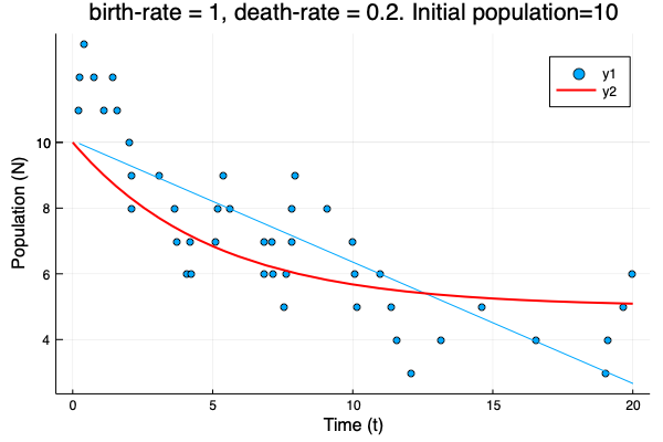
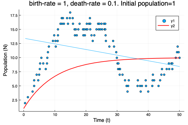
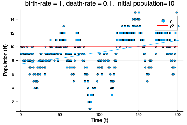
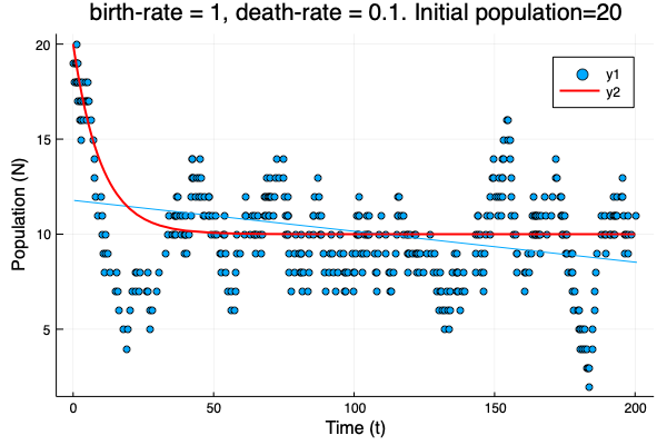
General equation, we obtain the asymptotic trend. With previous solution for the general problem: \(n=\beta/d\). The concavity will depend on the sign of \(C\).
Stochastic Simulation Algorithm
-
Two possible events might occur and these might happen at different rates: birth and death. \begin{equation} \frac{trial_{death}}{trial_{birth}+trial_{death}}= \frac{d\cdot N}{\beta + d\cdot N}, \qquad \frac{trial_{birth}}{trial_{death}+trial_{birth}}= \frac{\beta}{\beta + d\cdot N} \end{equation}
-
Bernoulli Trial. A event can either be a birth or a death. So we need to determine which event have actually occured. For this porpuse we choose a random number between \((0,1)\) and see if it is less than \(\frac{d\cdot N}{\beta + d\cdot N}\) or bigger. In each case we add or subtract an individual to the population (Monte-Carlo simulation).
-
For simplicity and to avoid divisions, we take a random number between \((0, d\cdot N+\beta)\), and we check that it is less than or greater than \(d\cdot N\).
-
Events in birth-death processes do not occur at regular time intervals. We can only say that the odds of an event occurring within any small time interval \(\Delta t\) is equal to \(a_{0} \Delta t\), where \(a_0\) is the mean rate of event occurrences. A sequence of random wait times is an example of what is called a “Poisson Process.”
-
Wait-times between sequential events follow an exponential distribution where the probability of the next event occurring after a duration \(\tau\) (give-or-take \(\Delta t\)) is given by:
\begin{equation} P(\tau) = a_{0} \cdot e^{-a_0 \cdot \tau} \end{equation}
- By superposition property we get that \(\tau = - \frac{\log{r}}{\beta + d\cdot x}\). Where \(r\) is a random number between \((0,1)\).
Results
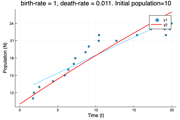
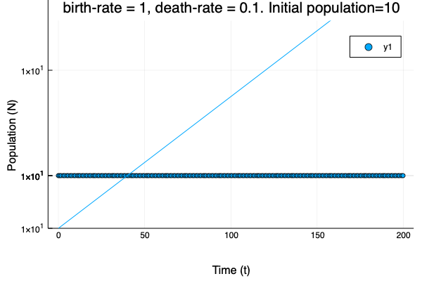
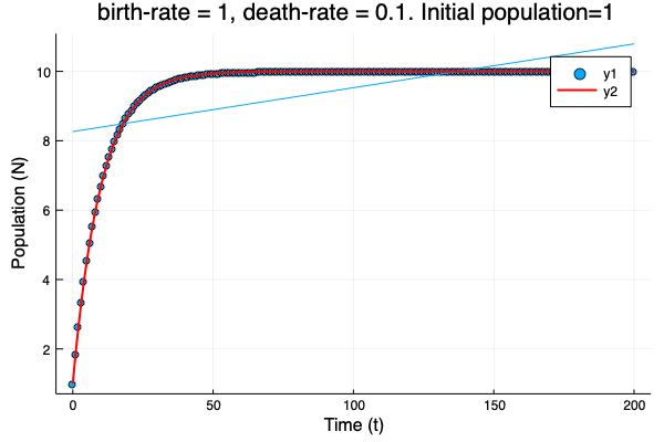
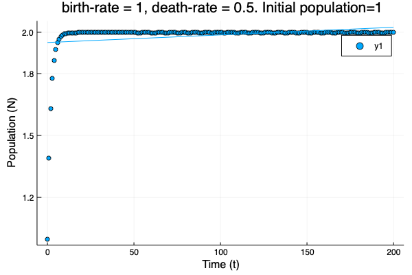
- We show different simulations (blue points) for different values of birth-rate and death-rate vs theoretical solution (red line). Blue line is the mean square approximation.
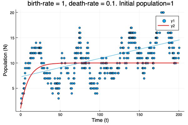
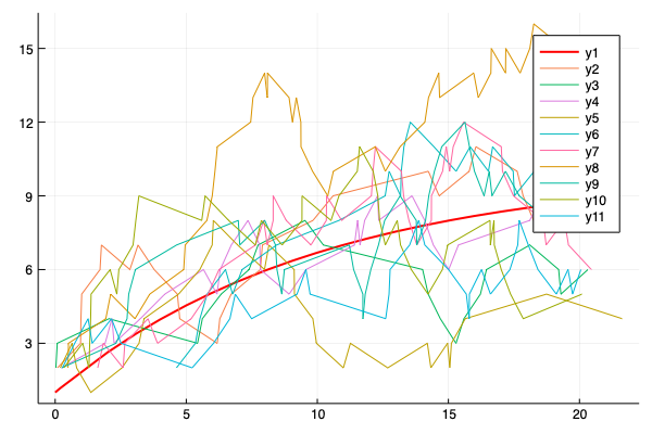
- Multiple simulations with same parameters vs theoretical solution (red bold line).
Installation
To install BirthDeathProcess, simply use Julia’s package manager. The module is not registered so you need to clone the repository and follow the following steps:
julia> push!(LOAD_PATH,pwd()) # You are in the BirthDeathProcess Repository
julia> using BirthDeathProcess
To reproduce the enviroment for compiling the repository:
(@v1.6) pkg> activate pathToRepository/BirthDeathProcess
Presentation
In the presentation folder, there is a beamer with a short presentation on the birth-death process and the implemented code.